Analyze multiple samples • CompassR

Example of CompassR analysis of the mouse Myh6 gene, which has important functions in cardiac muscle contraction and adult heart development. We selected a group of samples from different mouse tissues, including gastrocnemius, heart, hippocampus, and cerebral cortex, for visualization. For each sample, CompassR visualizes the expression of Myh6 gene and the genomic locations of Myh6-linked CREs whose chromatin accessibility is significantly associated with the gene expression of Myh6. CompassR also visualizes the genomic locations of the Myh6 gene and a union set of Myh6-linked CREs across all samples.

library(CompassR)

Load the data from CompassDB and extract the expression and linkage information for the Myh6.

## Example for Myh6 in mouse heart sample
expr_vec = query_exprssion("mm10", "Myh6")
link_res = query_linkage("mm10", "Myh6")

link_df = link_res[["linkage"]]
sample_df = na.omit(link_res[["samples"]])

sample_df = sample_df[sample_df$donor_gender == "Male", ]
sample_df = sample_df[, c("sample_id", "bio_source")]
colnames(sample_df) = c("Sample", "Group")
sample_df = sample_df[order(sample_df$Group), ]

link_df = link_df[link_df$sample %in% sample_df$Sample, ]

expr_df = data.frame(t(expr_vec)[sample_df$Sample, ])
colnames(expr_df) = c("Gene")
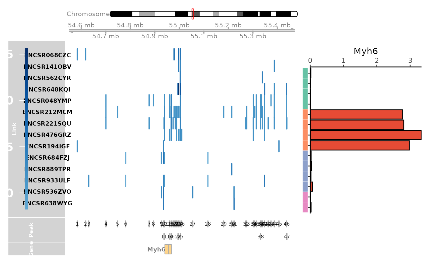
expr_df$Sample = rownames(expr_df)

Visuzalize the expression and linkage information for the Myh6 gene on samples of interest.

### This can fail when ensemble server is down, if that is the case, please try it later
link_df$sample_id = link_df$sample
genome_track_map(link_df, sample_df, "Myh6", expr_df, assembly = "mm10", legend.position="left", t = -20, b = 20)
#> the plot was flipped and the y limits will be applied to x-axis
#> Warning in get_plot_component(plot, "guide-box"): Multiple components found;
#> returning the first one. To return all, use `return_all = TRUE`.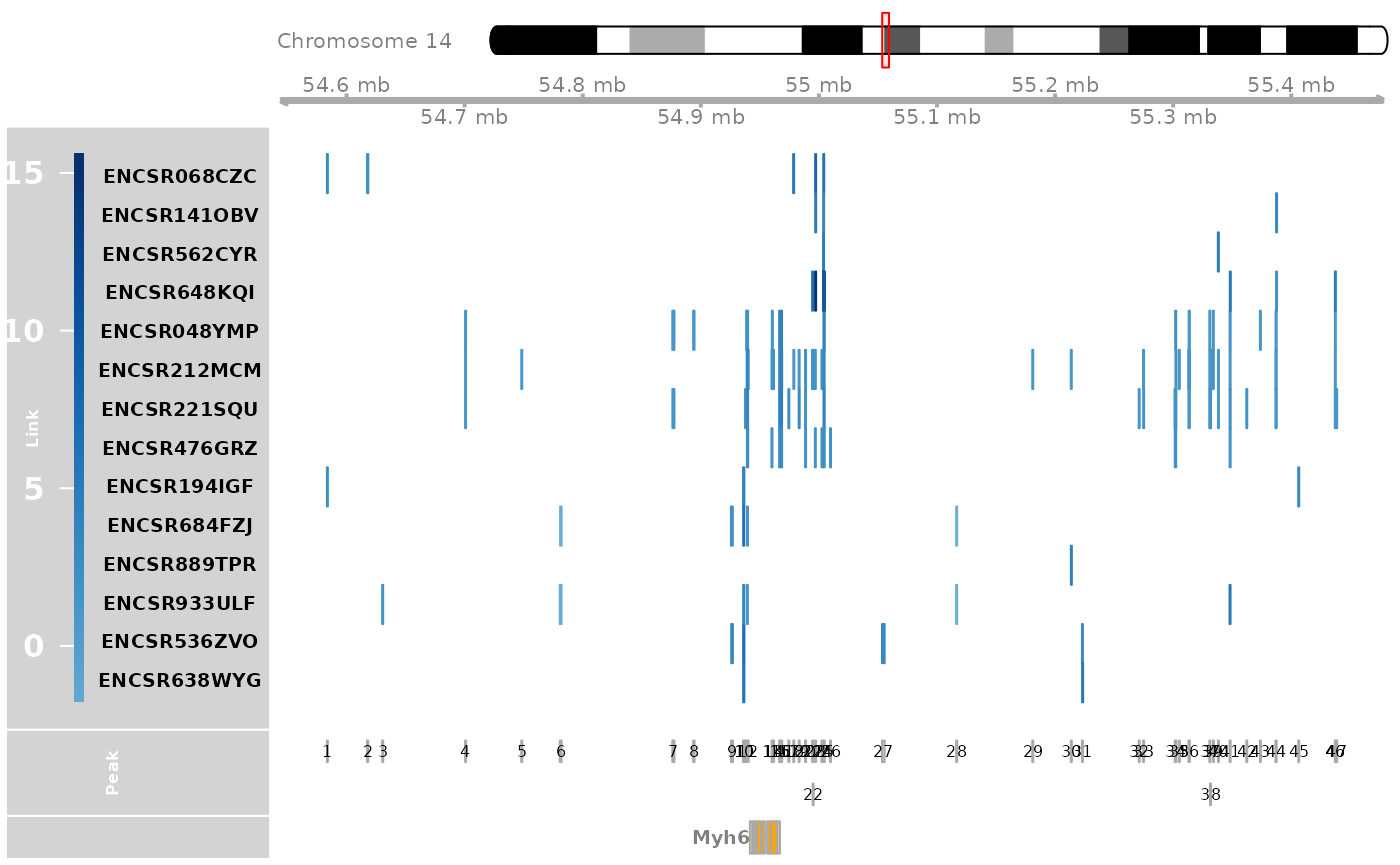

Extract the CREs linked to Myh6 expression in heart and plot the TF binding information.

track_plot = plot_genome_track(link_df, "Myh6", "mm10", sample_df$Sample)

peaks = track_plot[[length(track_plot)]]
peaks$name = as.character(peaks$name)
peak_order = make_peak_group(link_df, peaks, sample_df)

ht_peak_order = peak_order[peak_order[, "Heart"] >= 0.5 & peak_order[, "Gastrocnemius"]<0.5 & peak_order[, "Layer of hippocampus"]<0.5 & peak_order[, "Left cerebral cortex"]<0.5, ]
ht_peaks = rownames(ht_peak_order)

peak_vec = sub(":", "-", as.character(peaks))
ht_peaks = peak_vec[as.numeric(ht_peaks)]

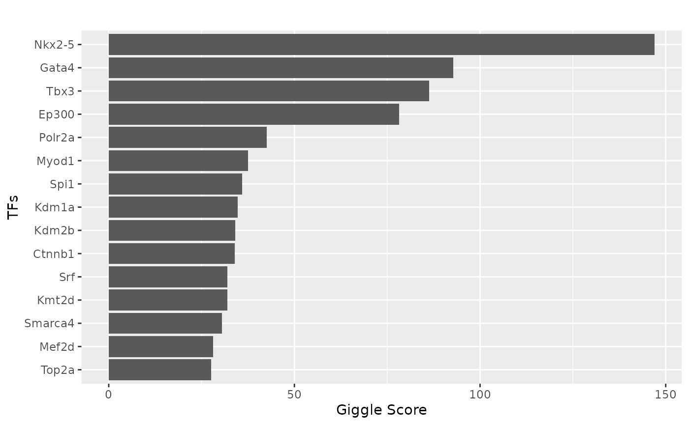
tf = tf_binding("mm10", paste0(ht_peaks, collapse = "_"))
plot_giggle(tf)